Using the Spreadsheet

From the View menu, hide the Algebra View and show the Spreadsheet View.  After showing the Spreadsheet View, you may have to click and drag the right edge of your screen to make the spreadsheet appear. Copy the data at the bottom of this tutorial and paste them into columns A and B.  (Select cell A1 then Ctrl-V)
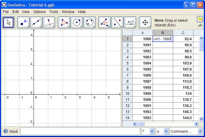
Right-click the heading of column B and select "Insert Left".  In cell B1 type    =A1 - 1980     then hit enter. Select cell B1, grab the "fill corner" on the bottom right of the cell, then drag it down to row 29, completing the table.
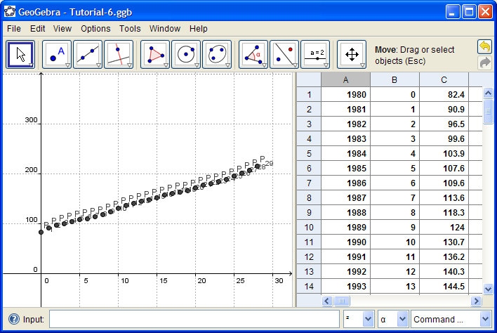
Select columns B and C, right-click, and choose "Create List of Points" Holding the shift key, drag the axes to change their scale and get the points into view.
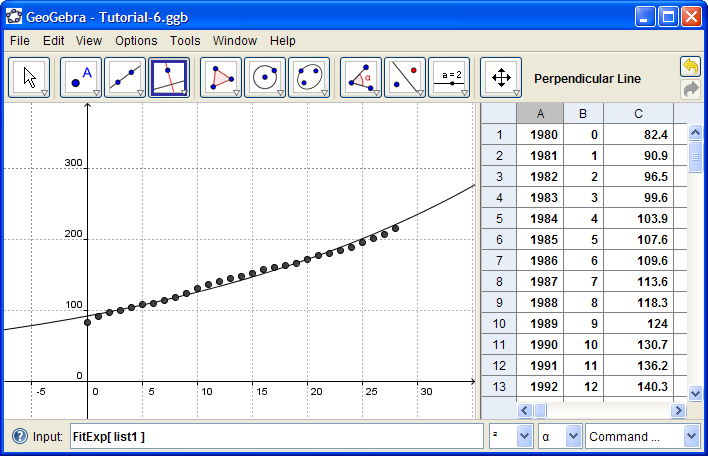
Enter the Object Properties dialogue box (Ctrl-E) select the points, and turn off their labels. If you look in the Algebra View, you'll see that the points are all gathered in a list, called  list1 .  Type the command   FitExp[ list1 ]  into the Input Bar. In the Algebra View you can get the equation of this graph. Browse through the command list; there are many statistics commands available that you can use with data in the spreadsheet.